Hi everyone! This week, I was traveling to Park City, Utah, to participate in the 3-week Park City Mathematics Institute. It’s currently a blast! I have more time now, but in the meantime, I asked my good friend Mike Schmidt to write a guest article for me. He wrote on probability which, if you’ve been reading for a while you know, is deeply connected to modern physics.

Anyway, here’s the article. Thanks, Mike!

The laws of Probability
So true in general
So fallacious in particular.
~Edward Gibson

 

Probability is just so fantastic, I could eat it all up. (Chocolate dice by Dice Candies).

Throughout history, humans have played games of chance. However, it wasn’t until the 1600s when Blaise Pascal and Pierre de Fermat started to investigate the a mathematical description of chance. The story starts, as most good stories do, with gambling. The following passage comes from Tom Apostol’s excellent calculus textbook:

“A gambler’s dispute in 1654 led to the creation of a mathematical theory of probability by two famous French mathematicians, Blaise Pascal and Pierre de Fermat. Antoine Gombaud, Chevalier de Méré, a French nobleman with an interest in gaming and gambling questions, called Pascal’s attention to an apparent contradiction concerning a popular dice game. The game consisted in throwing a pair of dice 24 times; the problem was to decide whether or not to bet even money on the occurrence of at least one “double six” during the 24 throws. A seemingly well-established gambling rule led de Méré to believe that betting on a double six in 24 throws would be profitable, but his own calculations indicated just the opposite.

This problem and others posed by de Méré led to an exchange of letters between Pascal and Fermat in which the fundamental principles of probability theory were formulated for the first time. Although a few special problems on games of chance had been solved by some Italian mathematicians in the 15th and 16th centuries, no general theory was developed before this famous correspondence.

The Dutch scientist Christian Huygens, a teacher of Leibniz, learned of this correspondence and shortly thereafter (in 1657) published the first book on probability; entitled De Ratiociniis in Ludo Aleae, it was a treatise on problems associated with gambling. Because of the inherent appeal of games of chance, probability theory soon became popular, and the subject developed rapidly during the 18th century. The major contributors during this period were Jakob Bernoulli (1654-1705) and Abraham de Moivre (1667-1754).

What does it mean to be random? If you do something the same way each time, but the outcome is different, that’s random. More formally, an operation which results in different results given identical starting conditions is said to be random. A random system, is the system where you perform the operation. For example, if I flip a coin, I’ve performed a random operation. But the coin is the random system.

Before the turn of the 20th century the predominant theory of the world was that of determinism. Determinism is the belief that if there is a set of initial conditions, there is only one result. Well, this would lead us to believe in a deterministic “clockwork” world; there would be no randomness.

At the time, our definition of randomness wasn’t really considered to be true. Instead, a system which exhibited severe sensitivity to initial conditions was considered to be random. Take for instance a coin flip; if you knew the exact force and direction imparted to the coin you could determine which face would fall upwards. Since there is always errors in measurement, there will aways be some level of uncertainty. In the coin example, there is so much sensitivity to initial force and direction, you could never be certain of where it would fall.

At the beginning of the 20th century, determinism started to seem incorrect. As evidence of quantum mechanics accumulated, notions of true randomness began to emerge. For the first time in physics, there was now evidence which competed directly with determinism. Quantum mechanics suggests there is no way, no matter how careful you are, to completely determine the outcome of an experiment.

(In fact, there was a recent paper arguing that even a coin flip is a quantum-mechanical effect, and inherently random. The paper was co-authored by Andreas Albrecht, one of the inventors of inflationary theory, and his student. There’s a nice article on it in new scientist, which is unfortunately behind a paywall. If you want, though, you can read the actual paper for free here.)

Upon hearing this, the situation seems pretty bleak, doesn’t it? Fortunately, the distinction between “I don’t know how this will pan out” and “I can’t know how this will pan out”  doesn’t really change the analysis! So, how exactly do we characterize a random outcome? Well, we can only express the likelihoods of specific outcomes.

Coin Flips

Let’s start looking at the most basic probabilistic system, the coin flip. If you flip a coin once, you’ll either get H(eads) or T(ails). Since each option is equally likely, the likelihood is 1/2 for heads or tails. Notice that 1/2 + 1/2 is 1. This is always a rule of probabilities: the sum of all likelihoods is one. In other words, this means that we require that something happen.

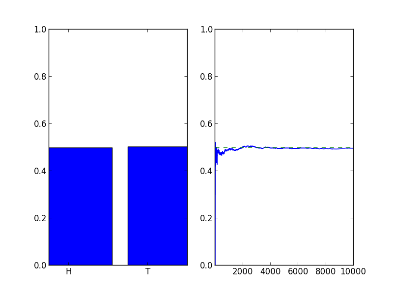
To show what this could look like, the following animation shows how a the counts add up over the course of many flips. The left plot shows the percent of flips that came out heads (left bar) and the percentage of tails (right bar) that have appeared as we flip the coins. The right plot shows the percentage of heads as a function of flips.

After many flips the chart will settle down to something that looks like this:

Now, let’s look at another coin flip, but this time let’s flip two coins! In this case there are four possible outcomes: HH HT TH TT. Again, since every option is equally as likely to occur, we say that each has a 1/4 chance to occur. In this case we’ve required what is called ordering. In other words, Coin 1 is distinct from Coin 2. What if we relaxed this requirement? That is to say, what if we threw both coins in the air and didn’t know which was which? In this case we couldn’t tell the difference between the HT and TH outcomes, they would be the same! Now we have a new situation, the outcomes are now: HH (HT or TH) TT. We only have three outcomes but the middle outcome is ambivalent of order. We’ll say the middle outcome has a weight of two.

This will change our arithmetic slightly; now the likelihood of an outcome is the weight/sum of weights. The sum of weights would be 1 + 2 + 1 = 4. Therefore, HH is 1/4, (HT or TH) is 1/2, and TT is 1/4.

Another way to think about it is to treat probability as a counting problem. The probability of getting a specific outcome is the number of ways that outcome can occur, divided by the total number of ways any outcome can occur. In the two coin flip example, there are two ways that you can get a head and a tails, TH or HT… and a total number of 4 outcomes. Then you get a probability of 2/4=1/2.

Let’s take another break and talk about what these likelihoods mean. A likelihood is, pedantically, the weight of a particular outcome compared to other outcomes. In the single coin flip example, heads and tails are equally weighted and are the only two options, so we can see the likelihood is 0.5 (as  0.5 + 0.5 = 1  ). Now, let’s consider what happens when there are unequal weights; suppose you have a special 6-sided dice where two sides are the same, say 1. There are 6 possible outcomes 1,1,2,3,4,5. We now say the likelihood of getting a 1 on a single role is 2/6 or 1/3. We can compare this to the likelihood of rolling a 2 which is 1/6.

Now, we may compare the two likelihoods and say that rolling a 1 is twice as likely as rolling any other number. Additionally, if we look at a set of trials, say six rolls, we will “expect” to see two ones, and one of each other number.

Now what does it mean to expect a specific outcome? Say we run a very large number of trials; on average, two 1’s will appear per trial, and each number will appear one time. So when we speak about the likelihood of an outcome, we are only making claims about what would happen on average if we ran the same trial many times.

What if I flip coin after another, and I want to know the probability of getting two heads in a row? We already know from counting that the answer will be 1/4. But is there another way to look at it? There sure is! If you do two random things, and they’re not related, then you can calculate the probability of one outcome happening after the other by multiplying the two probabilities. So, since the probability of getting H on a single coin flip is 1/2, the probability of getting H twice in a row is

   

Fun Examples

Since we now have a good understanding of basic probability, let’s lay out some things to think about.

First, one of the greatest unexpected answers from probability is the Birthday Problem.
The questions asks: what is the probability that two people in a room share a birthday? To answer this question it’s actually easier to first consider the opposite probability, the chance that in a room of n people, no two people share a birthday. To start, we know that there are only 365 days in a year and every person in a room has a birthday on one of those days. We start to build a probability distribution by looking at each person in the room. For the first person, we say their birthday can be on any day. For the second, if they do not share a birthday with the first person, we only have 364 days to then choose from. For the third, only 363. We can therefore see the probability that no one in the room shares a birthday looks like:

(1)  

If then the last term will be zero and will be zero! Now if we considered a room full of 365 people, we know it would be impossible to have no pair of two people who did not share a birthday, as we only have only 365 unique birthdays. So, the two ways of thinking fit with each other.

Now, what about the first question? The chance that no pair has a birthday and the chance that two do share a birthday must, when added, equal one. Therefore, we can say or where is the probability that out of n people, at least one pair share’s a birthday. Amazingly, if you compute it, ! This is quite astounding! On first look, 23 people sounds too low, but you must remember to consider the group as a whole where each pair must be considered.

Second, the Gambler’s fallacy is the belief that if you see a deviation from the expected likelihood in a small number of samples, that at some point the likelihood must over-correct to make up for the previous deviation. To see why this is untrue, we must remember two, say rolls of a dice, are independent. In other words, the outcome of the first roll doesn’t change the outcome of the second. This means there is no way for the dice to “know” it needs to correct and will therefore continue to play out with the same likelihood every time.

If you have any questions, as always, feel free to ask. If you have requests for additional topics, again, please post a comment asking for it.